Quality function
Q(s, a) → joint quality of state/action pair
根据 Markov decision process
Q(s, a) = E[ R(s’, s, a) + V(s’)] E对所有next state的 (R + V) 做加权平均
Quality of being in a state now = reward in the next state + value of next state
很重要的一点是我们默认所有value function, q function 都代表的是最大值
也就是s+1以后全部为最优路径
使这个值达到最优 也是我们优化Q func 的objective 但是我们首先就是要假设他们返回的就是最优
这种递归的写法统称就是bellman equation, 也叫动态规划方程, V = max_a(Q(s, a))

Without access to a model →
Monte Carlo learning
Purely through trial and error → episodic learning(play many sequence of a game)
requires a complete episode of interaction before updating our value function
像是玩游戏统计一条命 总共所做出的选择 和总收益
Compute cumulative award over episode
R_cum = 总共k step 的reward summation(+discount factor)
V_new(s) = V_old(s) + 1/n * (R_cum - V_old(s)) → For all particular states in this episode get the update(Basically the same without any bias for whether the individual state is good or bad)
这里为什么是 R_cum - V_old(s) → 因为 如果V_old 足够好的预测到了最终的value
那么R_cum 就可以被理解为该state的value
Temporal Difference(TD) learning
- specific optimal point in past associated with reward
TD(0) → V 可以观察下最主要和 Monte Carlo 的区别就是 与其走完整个episode
我们这里使用了这个bootstrap estimate 也就是这里的 TD target
作为预测的V(S_t) 把预测当前state值与预测 timestep t 后的值相挂钩

我们可以看到 learning rate 后面整个就是我们的 TD Error
我觉得另一种看待的方式是我们等于赋予了模型 跨越时间的能力 我们可以获取对S_t+n 的预测(这里可以把t+1 延展到 任意timestep之后 只需要在公式里加上对应State的discounted Reward)
并将他与S_t 所关联 这样如果我们S_t+1 相对准确的话 我们也就把这份精确度赋予了S_t的预测
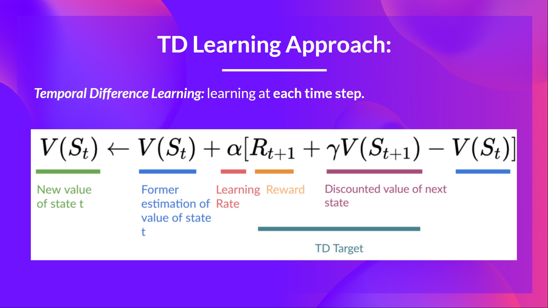
对于刚才我们说的t_t+n 我们还可以对n个timestep 的reward做加权平均 算总reward
然后把这个总reward当作 我们预测的S(t) 也就是TD target 对我们一开始V_old预测的计算差值

Q_learning → TD learning on the Q function

如我们所见 就是把之前的 V(s_t+1) 替换成了 Max Q(s_t+1)
这里面很重要的一点是 我们这里面所选择的action(我们可以看作是Behavior Policy)
不需要是maximize reward的 也就是必须符合我们Target Policy的
(其实也就是说eplison greedy)
Target Policy 永远跟从 Optimal path 也就是我们这里永远按最大值的方式算Q_value of next state
这个其实很好理解 基本上意思就是 允许我们走一些sub optimal step 但是对于S_t+1, 我们用max_Q 来获取他的最大value 这里也就是quality来表示
我们可以学习之前的经验 重复学习previous sample
对比的话我们来看
跟Q learning 的 off policy相反的 SARSA (State-Action-Reward-State-Action)
是On policy TD learning of the q function

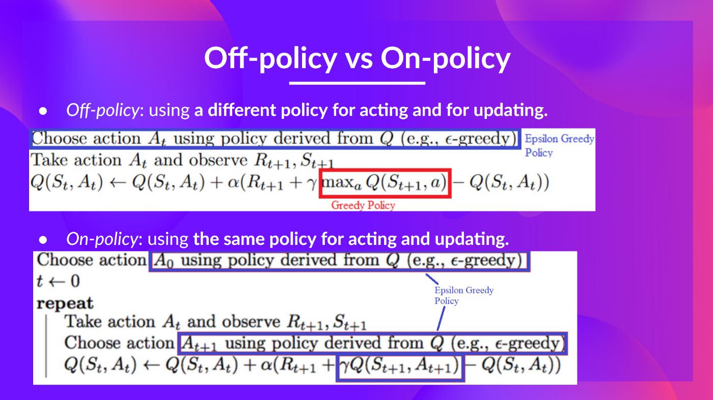
在这里我们所选择的 action 与我们来计算target q的action一致
有一种做了错误的选择但还是要硬着做下去的感觉 如果我们一开始跟着很差的Q function
有可能我们最后距离真实Q value 很远吗
这里我们只需要记得SARSA 的话其实就是 你选action其实跟Q learning 是一样的
都是epsilon greedy 都是允许 exploration
唯一的区别就是 我们这里使用 选action时所用的一样的policy (都是epsilon greedy举个例子)
这样保持我们policy的一致性
一个正确的认知是 我们现在都在谈论的value-based 我们是通过算q_value来判断这个S, t pair好不好
然后在此基础用一个func 这里广泛用的 epsilon greedy 来决定policy
这一段可以看https://huggingface.co/learn/deep-rl-course/unit2/q-learning 讲的非常清楚 感觉我有点没说的很好
最后代码实现可以看
https://gymnasium.farama.org/introduction/train_agent/
https://huggingface.co/learn/deep-rl-course/unit2/hands-on
这个hands-on部分很详细
参考:
https://huggingface.co/blog/deep-rl-q-part1
https://www.youtube.com/watch?v=0iqz4tcKN58&ab_channel=SteveBrunton